- How does Radio Echo Sounding Work?
- Frequencies and Wavelengths
- Instrumentation
- Radio Wave Propagation in Ice
- Field Work
- Data Processing
- Results
- Photos and Links
- References
How Does Radio-Echo Sounding Work?
A radio-echo sounding system consists of two main
components: 1) the transmitter, and 2) the receiver. The
transmitter sends out a brief burst of radio waves of a
specific frequency. The receiver detects the radio waves from
the transmitter and any waves that have bounced, or reflected
off nearby surfaces. The receiver records the amount of time
between the arrival of the transmitted wave and any reflected
waves as well as the strength of the waves (measured as an AC
voltage).
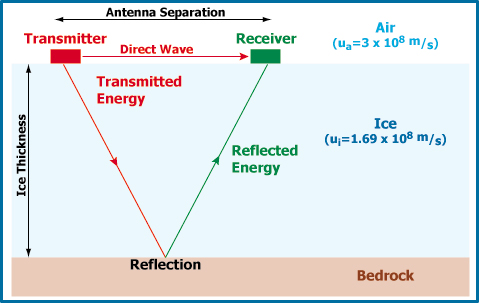
The radio waves travel at different speeds
through different materials. For example, radio waves travel
very close to 300,000,000 meters/second (3 x 10⁸ m/s) through air, a little less than double the speed in ice
at 1.69 x 10⁸ m/s.
See the next three tabs for more indepth explaination.
Frequencies & Wavelengths of Waves
Electro-Magnetic (EM) energy is made up of both particles
and waves. A single wavelength is 2¼ or 360° of
the wave's angular distance. When a wave travels through a
material, the wavelength is the distance travelled through
the material by 2¼ of a wave.

The number of times a wave oscillates over a certain
amount of time is know as the frequency of the wave.
The units of frequencies are Hertz (Hz) which is the number
of complete wavelengths that pass a point in a single second.
Therefore, 1 Hz = 1 cycle/second or 1/s.
The wavelength of a signal passing through a material
depends on the frequency (f ) of the wave and the
signal velocity (u ) through the material (a
property of the material itself). As shown above, the units
of frequency are 1/s, and the units of velocity are m/s.
Since wavelength(l ) is
measured in m, the equation to obtain wavelength is:
l = f * u
or wavelength = frequency * velocity
A higher amplitude wave of a
given frequency carries more energy than a low amplitude
wave. A signal can be detected only if its amplitude is
greater than that of any background noise. For example, if
you are listening to a radio in New York City, you can pick
up a station from Seattle only if its signal is stronger than
the EM noise caused by the sun, electric motors, local radio
stations, etc.
The Transmitter
There are numerous radio-echo sounding devices used by
various researchers thorughout the world. The components
described here are those used by researchers at the
University of Wyoming, which is based on that designed by
Barry Narod and Garry Clarke at the University of British
Coloumbia (Narod & Clarke, J. of Glaciology, 1995). It
has been designed for use on temperate glaciers.
The transmitter emits a 10 ns (nanosecond) long pulse at a
frequency of 100 MHz. The details of the pulse-generation
circuitry can be found in Narod & Clarke, 1995. The
frequency of the pulse is modulated for use on temperate
glaciers by attaching two 10 m antennas. The resulting 5 MHz
frequency is ideal for temperate glacier radio-echo sounding.
The transmitter is powered by a 12 V battery.
The transmitter and battery are housed in a small tackle
box which is attached to a pair of old skis. The antennas
extend out the front and back of the tackle box. The forward
antenna is carried by the person pulling the transmitter
sled's tow rope, while the rear antenna drags behind. There
is no focusing of the transmitted signal, so it propagates in
all directions into the ice and air. In order to reduce
"ringing" of the signal along the antenna,
resistors are embedded every meter along the antenna. The
total resistance of each 10 m antenna is 11 ohms.

The Receiver
The receiver begins with an antenna identical
to that of the transmitter. As each pulse is sent out of the
transmitter, some of the transmitted energy travels through
the air and some through the ice. The velocity of radio waves
in air is almost twice that in ice, so the receiver first
detects the "Direct Wave" transmitted through the
air between the transmitter and receiver. This triggers the
oscilloscope to begin recording the signal. For the next 10
µs, the oscilloscope records the voltage of the signals that
have reflected off nearby surfaces. The scope averages 64 of
the transmitter pulses and reflected waves to generate a
single trace. By averaging the scope reduces niose due to
signal scatter and instrument noise in order to obtain a
better trace to be recorded on the laptop computer. The
entire receiver is placed in a small sled which is pulled by
a tow rope. A third researcher monitors the signals on the
oscilloscope and records the information onto the laptop.
Both the scope and the laptop are powered by a 12 V battery
which can be charged by a solar panel for extended surveys.
Radio Wave Propagation in Temperate Ice
Background Information
As most people know, both water and ice are transparent to
the visible light portion of the Electro-Magnetic (EM)
spectrum. At the much lower frequencies (and longer
wavelengths) of radio waves, liquid water is opaque while ice
is still relatively transparent. This is why radio-echo
sounding is used in the sub-freezing regions of the Arctic
and Antarctic glaciers and ice sheets. There is little water
present within these cold ice masses to scatter or block the
radio signals. The lack of water has allowed researchers to
use frequencies ranging from a few MHz for subglacial
mapping, up to 200-500 MHz for crevasse detection near the
ice surface. Frequencies in the GHz range are used for
studies of snow structure and stratigraphy.
By definition, temperate ice exists at the
pressure-melting point. This means that both ice and water
phases coexist. The presence of liquid water presents a
problem when trying to use radio waves in temperate glaciers
because the water scatters the radio signals making it
difficult to receive coherent reflections that can later be
interpreted.
In the late 1960s through the mid-1970s, a number of
researchers experimented with various frequencies and
transmitter designs. Their findings concluded that
frequencies between ~2 and ~10 MHz are best for temperate
glaciers. 5 MHz pulse-transmitters are the most common used
today.
The basic reason that a 5 MHz signal works in most
temperate ice is that the resulting 34 m wavelength is far
larger than the size of the majority of the englacial water
bodies that scatter the signal. Unfortunately, the long
wavelength of the signal seriously limits the resolution of
the radio-echo sounding survey.
EM Wave Propagation Through a Dielectric Material
Radio waves travel through ice due to its dielectric
properties. The dielectric constant of a given material is a
complex number describing the comparison of the electrical
permittivity of a material and that of a vacuum. As a complex
number, the dielectric constant contains both real and
imaginary portions. The imaginary part of the number
represents the polarization of atoms in the material as the
EM energy passes through it (Feynman, 1964). The EM wave
propagation velocity is determined by its entire complex
dielectric constant.
The propagation velocity of a radio wave in ice is
determined by the dielectric properties of ice. Liquid water
and various types of bedrock have unique dielectric
constants. Since the dieliectric properties of a material are
related to conductivity, concentrations of dissolved ions in
liquid water will affect the dielectric constant (more free
ions increase the conductivity of water). The dielectric
constants of some materials are listed below:
| Material |
Dielectric Constant |
Reference |
| Air |
~1.0 |
Serway (1990) |
| Ice (at 0ºC) |
3.2 ± 0.03 |
Paren (Unpublished) |
| Water |
~80 |
Hasted (1961) |
| Quartz |
~4.3 |
Gregg (1980) |
Reflections of Waves
The Basic Concept
When a wave encounters an interface between materials of
different properties, the wave may be refracted, reflected,
or both. Snell's Law describes the reaction of light to a
boundary between materials of different dielectric contrasts
(or refractive index), based on the angle at which a ray
perpendicular to the wave front hits the interface. The angle
of the incoming ray (Angle of Incidence: ai)
is equal to the angle of reflection (ar).
The Angle of Refraction (aR)
is determined by the ratio of the sines of the Angle of
Incidence to the Angle of Refraction and the ratio of the
dielectric constants for the upper and lower layers (e1 and e2).

There is a point where the Angle of Incidence
is large enough (close to horizontal) that there is no
refraction. This is called the Angle of Critical Refraction
where all the incoming waves are either reflected or
refracted along the interface. Ay angles larger than the
Angle of Critical Refracion result in only reflection.
Radio-Echo Sounding in the Field
Introduction
The appropriate field methods for gathering Radio-Echo
Sounding (RES) data depend upon the objective of the survey.
If a researcher simply wants a rough estimate of the glacier
thickness, only a couple readings might suffice. If a
high-resolution map of the glacier bed is desired, a dense
grid of measurement points is necessary. Below is a
description of the field techniques used to develop a
high-resolution map of the glacier bed. It is important to
remember that even after the field work is over there are
many hours of data processing to be done. The techniques
described here were developed to minimize the processing time
and to maximize the resolution of the resulting map.
Mapping the RES Grid
When processing and interpreting the RES data after the
field season, the researcher needs to know the topography of
the glacier surface to correct for changes in the recorded
wave travel times. The glacier surface topography is mapped
using the Global Positioning System (GPS) or by traditional
optical surveying. While GPS is faster, it does not have the
vertical or horizontal resolution of optical surveying. The
horizontal positions are necessary to locate the map with
respect to other maps of the area, while the vertical
coordinates are critical for the data processing and need to
be accurate to within 0.5 m.
In order to reduce the possibility of spatial aliasing and
to maximize the resolution of the RES survey, the traces
should be recorded less than one-quarter wavelength apart.
For example, a 5 MHz RES system produces a 34 m wavelength.
Therefore the grid of RES traces should be less than 8.5 m
apart.
A rectangular grid with the traces aligned at 90° to one
another greatly simplifies the data processing.
Unfortunately, field conditions do not always oblige such an
orderly system and the grid is modified by the presence of
crevasses, melt-water ponds, steep slopes, avalanche debris,
etc. In such cases, detailed notes help to recreate the grid
during the data processing.
Recording the Profiles
The transmitter and receiver occupy separate sleds. These
may be pulled in-line or side-by-side depending on the design
specifications of the instruments. The Univ. of Wyoming
system is pulled side-by-side so that the transmitter and
receiver are pulled parallel to one another. A single
researcher pulls the transmitter on its homemade sled while
another pulls the receiver sled. A third researcher walks
beside the receiver sled to monitor the incoming signals on
the oscilloscope and then record them to the laptop computer.
Some systems can continuously record traces to a computer
and do minor amounts of pre-processing such as trace stacking
(or averaging) and digital filtering to remove noise. The
Univ. of Wyoming system is much simpler requiring the
researchers to stop at each position in the RES grid and
manually tell the computer to retrieve data from the
oscilloscope. Although more time consuming, this method
allows the researchers to monitor the condition of the
incoming data and results in a smaller data set. Each trace
recorded onto the computer is an average of at least 64
received pulses from the transmitter so that the
signal-to-noise ratio is improved.
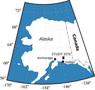
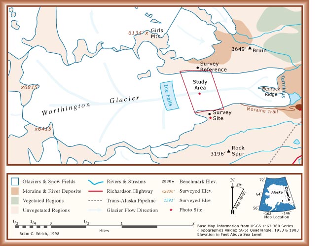
RES Field Work on the Worthington
Glacier, Alaska
The Worthington Glacier is a
small temperate valley glacier in the Chugach Mts. of
South-Central Alaska. Radio-echo sounding surveys have been
recorded there in support of ice-dynamics research by the Univ. of Wyoming and the Institute
of Arctic & Alpine Research at
the Univ.
of Colorado.
Processing Radio Echo-Sounding Data
Introduction
Processing the Radio Echo-Sounding (RES) data transforms
the data from incoherent numbers to a data set that can be
interpreted. Our processing methods are drawn from refection
seismology techniques. These are outlined in Welch, 1996; Welch et
al., 1998; and Yilmaz, 1987. We use a number of IDL (from
Research Systems, Inc.) scripts to organize our data and
usually create screen plots of each profile through each step
of the processing to help identify problems or mistakes. We
also use Seismic
Unix (SU), a collection of freeware seismic processing
scripts from the Colorado School of Mines. SU handles the
filtering, gain controls, RMS, and migration of the data. IDL
is used for file manipulation and plotting and provides a
general programming background for the processing.
The processing steps below are listed in the order that
they are applied. The steps should be followed in this order.
Note that quality of the processing results are strongly
dependent on the quality of the field data.
Data Cleaning and Sorting
The first step of data processing is to organize and clean
the field data so that all the profiles are oriented in the
same direction (South to North, for example), any duplicated
traces are deleted, profiles that were recorded in multiple
files are joined together, and surface coordinates are
assigned to each trace based on survey data. These steps are
some of the most tedious, but are critical for later
migration and interpretation.
Static and Elevation Corrections
The data is plotted as though the transmitter and receiver
were a single point and the glacier surface is a horizontal
plane. Since neither is the case, the data must be adjucted
to reflect actual conditions. The transmitter-receiver
separation results in a trigger-delay equivalent to the
travel-time of the signal across the distance separating the
two. This travel-time is added to the tops of all the traces
as a Static Correction.
The data is adjusted with respect to the highest trace
elevation in the profile array. Trace elevations are taken
from the survey data and the elevation difference between any
trace and the highest trace is converted into a travel-time
through ice by multiplying the elevation distance by the
radio-wave velocity in ice (1.69 x 10⁸ m/s). The
travel-time is added to the top of the trace, adjusting the
recorded data downward.
Filtering and Gain Controls
We use a bandpass filter in SU to elimitate low and high
frequency noise that result from the radar instrumentation,
nearby generators, etc. Generally we accept only frequencies
within a window of 4-7 MHz as our center transmitter
frequency is 5 MHz. Depending on the data, we will adjust the
gain on the data, but generally avoid any gain as it also
increases noise amplitude. We try to properly adjust gain
controls in the field so that later adjustment is
unnecessary.
Cross-Glacier Migration (2-D)
We 2-D migrate the data in the cross-glacier (or across
the dominent topography of the dataset) in order to remove
geometric errors introduced by the plotting method. Yilmaz
(1987) provides a good explanation for the need for migration
as well as descriptions of various migration algorithms.
Why is migration necessary?
The radar transmitter emits an omni-directional signal
that we can assume is roughly spherical in shape. As the wave
propagates outward from the transmitter, the size of the
spherical wavefront gets bigger so when it finally reflects
off a surface, that surface may be far from directly beneath
the transmitter. Since by convention, we plot the data as
though all reflections come from directly below the
transmitter, we have to adjust the data to show the
reflectors in their true positions.
We generally use a TK migration routine that is best for
single-velocity media where steep slopes are expected. As you
can see from the plot below, the shape of the bed reflector
has changed from the unmigrated plots shown in the previous
section.
Down-Glacier Migration (2-D)
In order to account for the 3-dimensional topography of
the glacier bed, we now migrate the profiles again, this time
in the down-glacier direction. We use the same migration
routine and the cross-glacier migrated profiles as the input.
Although not as accurate as a true 3-dimensional migration,
this two-pass method accounts for much of the regional
topography by migrating in two orthogonal directions. Radar Profile After Down-Glacier
Migration
Interpretating and Plotting the Bed Surface
Once the profiles have been migrated in both the
cross-glacier and down-glacier directions, we use IDL to plot
the profiles as an animation sequence. The animation shows
slices of the processed dataset in both the down-glacier and
cross-glacier direction. By animating the profiles, it is
easier to identify coherent reflection surfaces within the
dataset. Another IDL script allows the user to digitize,
grid, and plot reflection surfaces.
The resolution of an interpreted surface is a function of
the instrumentation, field techniques and processing methods.
Through modeling of synthetic radar profiles, we have shown
that under ideal circumstances, we can expect to resolve
features with a horizontal radius greater than or equal to
half the transmitter's wavelength in ice. So for a 5 MHz
system, we can expect to resolve features that are larger
than about 34 m across. Since the horizontal resolution is
far coarser than the vertical resolution of 1/4 wavelength,
we use the horizontal resolution as a smoothing window size
for the interpreted reflector surfaces. We use a
distance-weighted window to smooth the surfaces.

The ice and bedrock surfaces of a portion of the Worthington
Glacier obtained in the 1996 radio echo sounding survey. The 1994
boreholes are also plotted. (Plot by Joel Harper, U. of Wyo.)
Click on the image for a larger version.
The ice surface and bedrock surface beneath the Worthington
Glacier, Alaska. Resolution of both surfaces is 20 x 20 m. Yellow
lines indicate the positiond of boreholes used to measure ice
deformation.

Pictures of the Worthington Glacier Area
Notes on Radar Profiles
Three arrays of Radio-Echo Sounding profiles have been
recorded on the Worthington Glacier. The 1994 survey was recorded
using different field methods than the field methods used in 1996
& 1998. The same eqpuipmet was used in all three surveys as
well as the same data processing techniques.
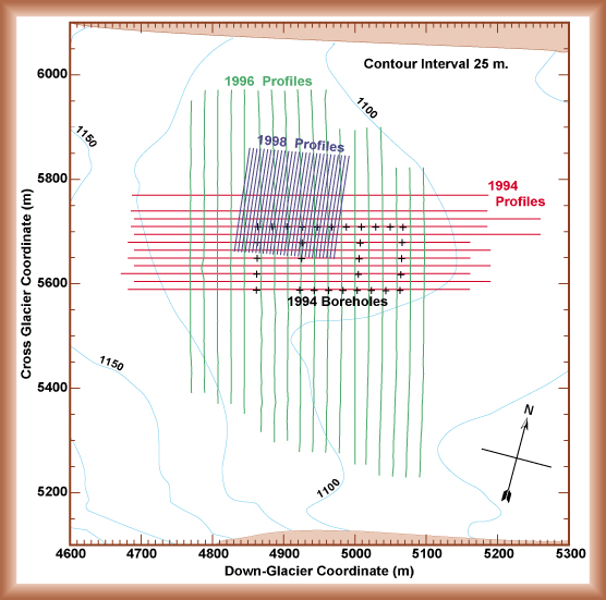
1994 Survey
The first profiles were recorded in 1994 and oriented
parallel to the ice flow direction. The locations of these
profiles were not measured accurately, and the profiles were
recorded a few at a time over a period of about a month. The
resulting glacier bed map was not very accurate, with a
resolution of about 40 x 40 meters.
1996 Survey
The 1996 radar profiles were recorded in the cross-glacier
direction. The location of every fourth trace of each profile
was measured with optical surveying equipment using a local coordinate system seen in the map
below. The profiles were spaced 20 m apart and a trace
recorded every 5 m along each profile. The resulting glacier
bed map had a resolution of 20 x 20 meters.
1998 Survey
In 1998 we used the radio-echo sounding equipment to look
for englacial conduits that transport surface meltwater
through the glacier to its bed. This study required the
maximum resolution that we could obtain from the eqpuipment,
so the profiles and traces were spaced every 5 m. Every
fourth trace on each profile was surveyed to locate it to
within 0.25 m and the entire RES survey was recorded in two
days. The survey was repeated a month later to look for
changes in the geometry of any englacial conduits found. The
first RES survey was processed to produce a map of the
glacier bed surface with a resolution of 17.5 x 17.5 m. The
maximum resolution obtainable by an RES survey is half of the
signal wavelength. Our 5 MHz system, therefore, can obtain 17
x 17 m resolution under the best of circumstances.
Content 2
|